Goal
Background: In order to better understand the effect that drainage area has on a watershed, processes were conducted in order to delineate the watershed, determine its drainage size, slope, and use that data to create charts. ArcMap was used to delineate the Willow Creek Watershed, illustrate its boundaries, and trace the path of the main stem and northeast stem of the creek. Microsoft Excel was used to organize all of the information gathered from ArcMap and to create charts to show visual representations of the data. The results yielded similar numbers to the drainage area delineated by hand in a prior class exercise.
Introduction
This assignment focused on the Willow Creek Watershed, located south by southeast of the city of Eau Claire (Figure 1). After examining this watershed first hand, it was examined via topographic maps, in order to further break down the watershed and understand certain attributes. In order to better understand these attributes, the use of ArcMap 10.2 and Microsoft Excel was implemented to break down key figures, concerning drainage area, elevation, and slope. Using these methods, the ability to delineate this watershed was gained, long profiles were created to illustrate the shape of the creek, and various charts were constructed to illustrate these findings.
Methods
This research team consisted of Cody Kroening, who read and interpreted the instructions, Simon Dowling, who helped interpret the directions and check for errors, and the author of this paper, who performed the tasks instructed to him by Cody and Sean on ArcMap, and Excel. The first task was to load the appropriate files to ArcMap that would be used to start delineating the watershed of Willow Creek. After the initial tiff and shapefile were added, a personal geodatabase was created in ArcCatalog, named “WillowCk-hilgenzt”, for the purpose of storing all of the data in one file. After this, a map that had been delineated by hand, in class, was used to delineate the seven subsections of the Willow Creek Watershed. In order to carry out this task, first the full extent of the watershed was delineated using a hollow polygon feature to denote its boundaries. For each of the following delineations, labeled Wshed_A – Wshed_G, the original polygon, Wshed_A was copied and pasted as a new polygon feature class. Then the new feature class was labeled with the appropriate name and the “Cut Polygon” tool was used to delineate it to its proper size. The excess from the original polygon was deleted and only the smaller watershed remained. The process was repeated for all of the watersheds in order to get accurate matching borders for each.
After delineating all of the watersheds Microsoft Excel was launched and the project was labeled “SlopeAreaData”. Column 1 listed all of the watersheds, while Row 1 listed Drainage Area (m2) and Drainage Area (km2). The respective areas were found in the attribute table in ArcMap and they were recorded in Excel. A simple formula was created to create meters to kilometers and those figures were recorded as well. Then, the course of the creek was delineated. In order to do this, a line feature was added to the geodatabase labeled “WillowMainStem”. The editor toolbar was activated and the new line feature was selected. Starting at the first contour line, a line was created in segments, directly following the flow of the creek. At each contour line the segment was ended and a new one was started. This process repeated for the rest of the main stem. At certain points the creek flowed under roads, in which case the contour line denoting the road was ignored and the line was finished at the next contour. The same process was carried out for the northeast branch of the creek. The line feature was created and the creek was fully delineated. Then the data added to the “SlopeAreaData” spreadsheet under the column Segment Length, for both stems of the creek. Elevation Change (ft) and Elevation Change (m) was added to the spreadsheet and this data was recorded for each segment. This number was constant for each segment at 20 feet and 6.096 meters. Slope (m/m) was added and determined for each watershed by dividing the elevation change in meters by the segment length in meters. A chart was created to show this data by comparing the Slope (m/m) and Drainage Area (km2) columns. This data was fitted to a scatter chart, axis labels were added, and a trendline was fitted with equations and an (r2) value.
Finally, data from the WIllowMainStem line feature class was exported from ArcMap, as a dBase file, and was opened up in Microsoft Excel. This data contained the columns: Segment Length (m), Downstream Distance (m), Downstream Distance (km), elevation (ft), and elevation (m). All of this data was entered and simple formulas were created to quickly calculate conversions. A scatter chart with smooth lines and markers was created to illustrate the Long Profile of the stream as it flowed downstream. The same process was used for the northeast branch of the creek.
Results
Results
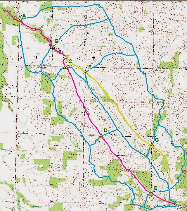
The data that this project yielded managed to provide very informative illustrations and data to better understand stream shape and dimensions. Through working in ArcMap, a better understanding of the shape and boundaries of watersheds was gained. The delineation of a watershed by hand can be very time consuming and inaccurate, so the ability to use a computer program to delineate provided a very accurate and precise resource. As stated in the previous section, the entire watershed was divided seven times, into smaller subsections from Watershed A (largest) to Watershed E (smallest) for the main stem, and from Watershed F (largest) to Watershed G (smallest) for the northeast stem, which can be seen in Figure 2. Following this, the line feature was used to highlight the course of Willow Creek (Figure 3).
The delineation data was transferred and expanded upon in Microsoft Excel. The first Excel Worksheet examined the slope of Willow Creek over its watershed. Slope was calculated by dividing the elevation change in meters by the drainage area in meters. Due to the fact that the segments of the watershed were collected from contour line to contour line, the slope was a constant number of 6.096 meters. The drainage area followed the pattern of decreasing from Watershed A-E and Watershed F-G. The entire watershed measured 9975654.029735 m2, or 9.97 km2. This data was used to create a chart that compared the slope of Willow Creek to its Drainage Area (km). An equation of y = 0.0131x - 0.405 was created by Excel to determine the comparison value. The (R2) value was a 0.93308, which exhibits a decently fitted trendline (Chart 1).
The next worksheet was created to determine the long profile of Willow Creek. Segment Length, Downstream Distance, and Elevation were listed in order to create a chart that illustrated the Long Profile. In this case, a long profile shows a linear approximation of the shape of Willow Creek as it flows downstream. The chart was comprised of a vertical axis, denoting Elevation (m), and a horizontal axis, denoting Downstream Distance (km). As shown in Chart 2, the model of the creek as it flows downwards is initially quite steep, leveling off gradually as it decreases in elevation in a concave upwards fashion. The same process was carried out for the northeast stem of Willow Creek. The results were much similar, though the initial decrease in elevation was not as extreme as was seen in the main stem profile (Chart 3).
Discussion
Discussion
The data and results gathered from this project matched expectations with what was anticipated to be found. The data that was collected from referencing ArcMap was actually rather close to the number this group gathered from its in class delineation. The hand drawn delineation of the entire drainage area yielded a number of 9.69408 km2, while the data interpreted in Excel was 9.97565403 km2, a relatively close correlation given that this data was approximated by hand initially. This was a relatively easy assignment and through it a better understanding of the processes of Microsoft Excel and ArcMap was achieved.
Conclusion
This assignment helped to illustrate the characteristics of the Willow Creek Watershed. Through the use of ArcMap and Microsoft Excel, this group was able to delineate, approximate, and analyze data provided by carrying out the methods described in this report. The results yielded information that was quite similar to the hand delineation assignment completed in class, which helped to further inform the group that their method was correct. This assignment was able to further the understanding of a watershed, its characteristics, and how to break a watershed down and analyze it.
Figures

 |
| Figure 1: This figure outlines the location and size of the Willow Creek Watershed. This watershed is located just southeast of Eau Claire, Wisconsin. |
 |
| Figure 2: This map shows the various watershed divisions examined in this assignment. The main stem consists of Watersheds A-E, while the northeast branch consists of Watersheds F-G. |
 |
| Figure 3: This map shows the main stem, as the fuschia-colored line, and the northeast stem, as the golden-colored line. The watershed is outlined. |
 |
| Chart 1: This chart shows the slope of Willow Creek in comparison to its drainage area in square kilometers. |
 |
| Chart 2: This chart shows a long profile of the northeast stem of Willow Creek. |
 |
| Chart 3: This chart shows a long profile of the northeast stem of Willow Creek |
No comments:
Post a Comment